AoC 2018 with Mathematica Reflection
William John Holden
2018-12-30
Advent of Code
Advent of Code (https://www.adventofcode.com) is a series of competitive programming puzzles created by Eric Wastl. I somehow stumbled across AoC late last year, had a lot of fun, and looked forward to participating again in 2018 all year. In 2017 I earned 25 stars in total after a late start. I used PowerShell at first but quickly switched to programming in Java. In 2017 I used any tool that felt well-suited to the problem; I used PowerShell, C, Java, Excel, GraphViz, and even pencil and paper. I got a late start in 2017 and ended on Christmas day with 25 total stars.
This year I took AoC as an opportunity to explore Mathematica. I started on day 1 and ended with 30 stars. Life happened and I had to take about a week break after December 5 or so but from December 18-24 I found a lot of time to work on these challenges.
I learned a lot about Mathematica and functional programming from this experience. This paper is intended to share my experience to those interested and document my findings for my own reference later.
I have a undergraduate degree in computer science but I have never worked as a professional programmer. I rate myself as an average programmer at best due to inexperience. Another AoC participant by the handle agent_who _glows used Mathematica; his or her solutions are immeasurably superior to mine.
My first general observation is that AoC 2018 was much harder than AoC 2017. I am not alone feeling this way (https://www.reddit.com/r/adventofcode/comments/a95eou/2018_harder _than _ 2017/). Fewer of the problems had a clever mathematical solution you could derive on paper or with OEIS (https://twitter.com/wjholdentech/status/944069093413359616) and more problems required you to simulate some kind of system. Unfortunately for me, Mathematica seems poorly suited to the simulations that were common to AoC 2018.
Mathematica is a functional programming language. In a functional programming language a pure function accepts parameters and returns a deterministic result with no side effects. (Mathematica isn’t purely functional. You can still built mutable data structures and whatnot, but the functional paradigm is central to Mathematica’s design and usage.) The functional approach has strengths and weaknesses. I am not an expert but I will share my limited insights from AoC.
Suppose you needed to implement a particle simulation where a fixed number of particles are translated from a starting position. A Java, C++, or Python programmer might reach for the object-oriented approach. Each particle would be its own object; the position data and translation behavior would be part of the particle instance. A C programmer taking an procedural approach might put the positions and behavior of each particle stored in arrays and then mutate the positions with a routine. The functional approach, preferred with Mathematica, accepts a stateless list of particles and time; the function would return the position of each particle after that amount of time has elapsed. The use of any approach with any particular programming language is only a generalization; all approaches are possible with all languages, but some are easier and more popular in one environment than another.
The functional approach to the above particle simulation problem has a couple of advantages. The stateless nature of the function lends to determinism, reproducibility, and verification. You shouldn’t end up with a “God object” in a functional program. Performance can be a problem, though. If the particle simulation can use simple multiplication to translate the particles then it probably runs in O(n). If the simulation has to iteratively increment and check values then it probably runs in O(t n) (where t is the time parameter), and this might be even worse if we have to perform collision detection at each frame. Repeating an O(t n) process t times obviously produces an  total time.
A functional particle simulator doesn’t have to compute the position from start to finish each time, though. The function might “tick” the simulation once, return the result, and then invoke the same function on the output. This is known as folding in functional programming. Mathematica has several functions for folding; in this case the Nest function is best suited to the problem. Returning a new list with each “tick” can be very slow because operations do not occur in-place; all new lists require memory operations. The following three functions give the same results for nonnegative integer t.


This toy example shows several interesting features of Mathematica. First, notice in the translateMultiply function that we can multiply a scalar to a vector (v t) and then add it to another vector (p) to get an intuitive answer. Mathematica handles all of the messy looping and assignments for us, which is nice. The translateIterative function uses a standard For loop in a way familiar to every C and Java programmer in the world. We want our problems to have easy solutions like the multiplication algorithm, but if all programming were this easy none of us would have jobs. The translateFold function achieves precisely the same result but conceals all of the bookkeeping. The # symbol is called “slot” and is semantically similar to Perl’s $_ operator. It gives access to parameters provided to a function.
Iterating through lists and returning a resulting list of the same size is also made easy with Mathematica. The Map function iterates through a list, performs some function on each element, and returns the resulting list. Map does not mutate the input list. Applying a function against each element of a list will feel familiar to anyone who has used Java’s Streams API.


I found myself using Map, Range, and Total all the time in AoC. Mathematica comes with a vast library of built-in functions that serve many purposes.
Day 1
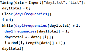
The first interesting lesson I learned was from day 1 (https://mathematica.stackexchange.com/questions/187131/improving-performance-of-algorithm-to-compute-code-puzzles).
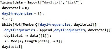
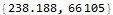
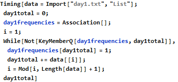
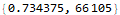
This program works, but it takes almost four minutes to complete on my computer. This is because the Append function requires O(n) time to create a new array of length n+1. This is a good example of where the purely functional approach fails. We need a mutable data structure that allows for faster insertions. One such data structure is Mathematica’s Association. Association is similar to the Map interface in the Java Collections Framework. Switching from an ordinary list to an Association significantly improves the performance of this algorithm.
An even faster method is to use something strange called down values. Mathematica’s syntax allows you to directly enter a value as part of a function definition.


Global`fibonacci
| fibonacci[1]=1 |
| |
| fibonacci[2]=1 |
| |
| fibonacci[n_]:=fibonacci[n-1]+fibonacci[n-2] |
|


These “down values” must be stored in some data structure that offers even faster lookups than an Association. In this program we treat day1frequencies as a function and write new down values to its definition.

Day 2
Mathematica’s functions allow for a short, simple, and fairly intuitive solution for day 2. These short programs took me quite a while to write! In the first problem we need count the number of strings in an input with exactly two or exactly three of any letter, then multiply these counts.


This program finishes so quickly that I am not interested in searching for efficiencies. From the inside out, we split an input string into a list of Characters.


Once we have a list of characters to work with we tally them up with the Counts function. We could have easily used Tally instead; the difference in these two functions is that Tally returns a two-dimensional array and Counts returns an association.


Now we Select the letters with a count equal to two or three. Mathematica uses the familiar “=” for right-to-left assignment and doubled “==” to test equality.


In this program we only care if a string contained duplicates or not. I used a simple If statement to turn our selection into ones and zeros. We use Map to apply all of this against each element of our input and Total to sum the ones and zeros.
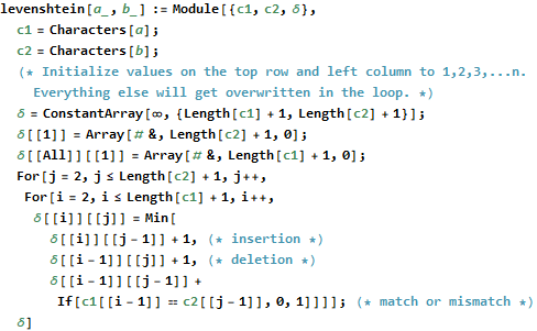
In part 2 we are prompted to find the pair within our input with minimum Levenshtein distance (aka editing distance) of exactly one. The problem does not use these terms and I might not have been able to solve this program had I not encountered editing distance in an edX class I attended last year.
The editing distance between two strings is the minimum number of insertions, deletions, and substitutions needed to transform one string into another. For example, “mello” and “yellow” obviously have an editing distance of 2; we just need to remove the “m” and “w”. The words “dynamic” and “programming” have a large editing distance of 8; we have mismatch or remove the substrings “progr”, “m”, and “ng” from the longer word.
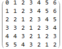
The editing distance problem is canonically solved with a dynamic programming algorithm that constructs a matrix of matches and mismatches. Here we weight insertions, deletions, and mismatches all with a cost of one and matches with a cost of zero. This is a pretty tricky algorithm to learn even in the classroom; I strongly doubt I could have come up with something this efficient on my own.


Mathematica already has a built-in EditDistance function.


My first solution for day 2 part 2 used Mathematica’s Scan function and a Print statement. This works well, but it reflects an ingrained Java mentality.


The functional approach is to map and reduce. Here is another Mathematica function that gives the same answer. The performance difference is unimportant.


Day 3
I don’t think that I have mentioned that on many of these projects I modified the input in Notepad or Excel to make it easier to import. In this program I removed all of the symbols in the input to create a bare table of comma-separated values.
Day 3 asks us to first find the count of overlapping integer points in a plane given a list of rectangular areas. Mathematica’s unusual syntax turned out to be very well-suited to this task.

We initialize a 1000×1000 zero matrix m. For each rectangle defined by our input we find the submatrix of m corresponding to these coordinates and allow Mathematica’s ++ operator to increment the value in each cell. The ConstantArray data structure is an instance of SparseArray and does not store a value for each element. The #[[1]] syntax refers to the position in the list passed to the function by Scan.
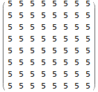
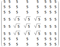
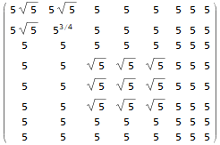
This syntax is interesting, subtle, and powerful. A simpler example follows. Begin with a constant array of fives named x. Take the square root of each element in the submatrix rows 4-6 and columns 3-5 and assign these values to y. Last, raise values to the 3/2 power from submatrix of y rows 3-4 and columns 2-3, but store these values in rows 1-2 and columns 1-2 of matrix z.
Day 4
The difficulty kicked up on day 4 and Mathematica was not well-suited to this problem. This would have been bread-and-butter in Java or Python.
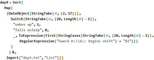
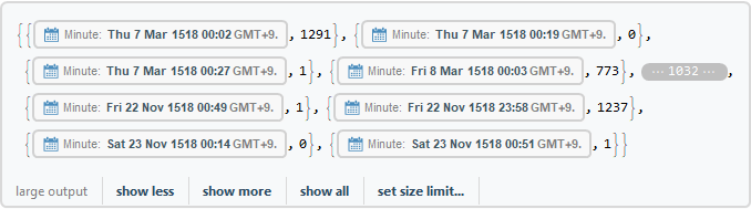
Read each line of text from input. Split the string into the date and then rest of it. We can do this the easy way, with absolute string indices, since fields within the strings have constant width. DateObject can recognize the ISO-8601 format directly. We parse the second half of the string as a 1 if the guard wakes up and 0 if the guard goes to sleep. For shift changes we match “_” (a pattern matching any expression) and get the guard number. StringCases returns an array so get the first, and only, element from this list. Finally, sort the entire thing.
Start with an association that will hold an array for each guard. The contents of the array represent each minute a guard might be asleep. Next iterate through the calendar, taking care not to double-count the last entry. If the second element in the calendar is greater than one then we are changing the guard and initializing the state to 1 (awake). If this guard has not been added to the sleep tracker then initialize it. If the state transitions to zero (asleep) then find the time the guard went to sleep and the time of the next element. An unstated invariant in the input is that guards always wake up before 1am. Increment the sleep counter for all minutes between the sleeping and waking times on the closed/open interval [start,stop). Sort the data structure by the total number of minutes spent sleeping. (This actually isn’t a perfect statistical metric for finding the sleepiest guard; what if the guard simply worked more shifts?) Print the position (minutes 1, because Mathematica is one-indexed) of the sleepiest minutes of the sleepiest guard.

Mathematica has many convenient features for scientific analysis. One such feature that is neat, but not particularly useful, for day 3 is to visualize the intervals directly.

With some effort one could color-code these intervals for each guard.
The second portion of day 4 was very easy once with the “minutes” stored in the earlier data structure.


Day 5
Day 5 was also quite difficult in Mathematica. Mathematica does not have its own stack or linked list data structures. You can build your own and this problem would look very much like the classic matching parentheses problem taught in schools.
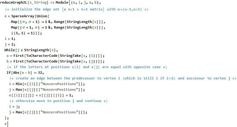
After much thought I realized that this problem can be viewed as contracting vertices of a graph. I construct an adjacency matrix for a graph, short-circuit edges with matching vertices, backtrack (to a minimum position 1) after contractions and advance otherwise. I reformat the input as positive and negative integers.


Reducing “exampleEXAMPLE” removes only the matched pair (5,-5) at the center.


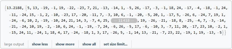


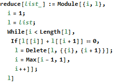
This algorithm is strange, slow, and confusing. Doubling the input, as shown below for a single case, increases the total running time by a factor of three. Use of the Delete function poses the same amortized  performance penalty that we saw on day 1, but on this day I was more interested in finding any solution than finding a quick solution.

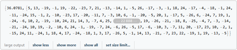
We can obtain the same result in only slightly less time by constructing the (n+1)×(n+1) matrix described earlier. I’m not exactly sure where the performance bottleneck comes from. I think I’ve probably earned the “most obscure and inefficient algorithm to do something obvious” award for day 5.

The graph is not visually interesting.


Solving part 2 is fairly straightforward but uses some unusual syntax. Here I create an anonymous function with Function. The reason for this is to explicitly name its parameter, “exclude,” because I also need the implicit parameter “#” for the selection statement. The following line says that for each integer i from 1 to 26, select only the integers in the list named “day5” that are not equal to ±i.

Now that we have these 26 lists (of unequal size), apply the reduce function to each list.


Day 6
AoC had a couple of Manhattan distance questions last year and they are back in force in 2018. Manhattan distance differs from Euclidean distance by taking discrete steps in a single direction.

Manhattan distance is very easy to calculate. You just add the absolute value of the differences between x and y for each coordinate. Of mathematical interest, notice that the Manhattan distance does not change with the number of subdivisions -- ever! You cannot take a limit of the below function and end up with the Euclidean distance formula.


So all that buildup...and Mathematica already has a built-in ManhattanDistance function.


We are prompted to construct a Voronoi diagram from a list of points.

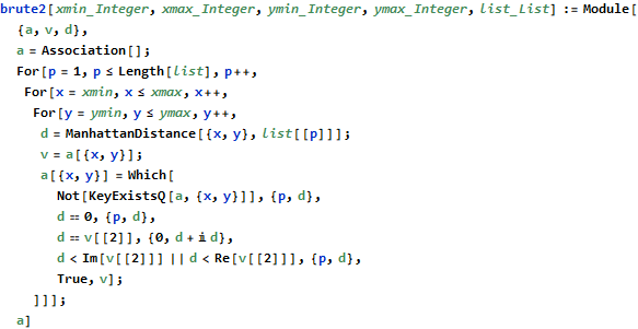
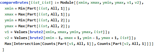
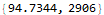
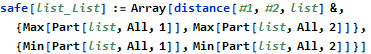
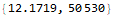
Several of the problems before were difficult to program, but this one was difficult from an algorithmic perspective. I couldn’t think of a way to detect the infinite points geometrically so I came up with a heuristic solution. Step 1 is to brute force the Manhattan distances in the bounding box defined by {xmin,xmax} × {ymin,ymax}. Next, brute force the Manhattan distances a second time in a bounding box defined by {xmin-1,xmax+1} × {ymin-1,ymax+1}. Find the intersection of these sets. The maximum element in the intersection is the solution in part 1. This program is very slow.
The brute forcing algorithm uses imaginary numbers to indicate an unusable tie. At first I was setting a tie to a large distance value (Infinity) but then a later point that is actually farther than the tied distance would overwrite it. I tried using a sentinel value of “.” for the “p” value but for some reason I had trouble getting this to work (go figure, complex numbers are easier than string comparisons in WolfLang).


In part 2 the requirement is inverted; we want to minimize the distance instead of maximizing it.


This algorithm has no overlapping subproblems. We can run it in parallel and reduce the computation time. (Strangely, this did not seem to help when I first wrote this program. Maybe I made a mistake on the first attempt.)


Day 8
I struggled with day 8 (https://twitter.com/wjholdentech/status/1076419523383721984). I ended up solving this problem in Java. Both programs were ugly and uninteresting.
Day 10
Day 10 was a great day for Mathematica! This program is a particle simulation. We don’t have to worry about collisions or nonlinear paths; to calculate the translated position we simply scale the velocity vector and add. Mathematica’s graphical features really shine here.

It took me much longer to actually find the interesting time (10227) than it took to build this graphic. Others noticed that the solution fits in the minimum bounding box for all values t∈Z. I didn’t realize this explicitly but I did find that the shape formed by these plots remains constant as t becomes large. I bisected values of t to find the region where t does something interesting.
Day 11
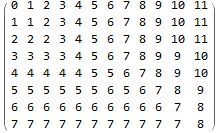
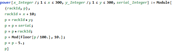
In day 11 we are given function to calculate power values in a 300×300 grid. The first part has us find the maximum value in this grid. This is pretty obvious O(n) problem. Mathematica has features to find the maxima/minima for a function but I never figured out how to use these. The solution that lept to my mind was to precompute the power output for each cell in the grid and then find the maximum value for a 3×3 region.


Graphics are not very useful for this problem.


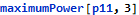
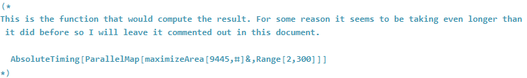
That was quick and easy. This approach should easily scale to find the maximum submatrix sum for all n×n grids within the region, right? Well, no. I first thought that we could run ParallelMap against maximumPower over the range 1 to 300, but this solution is very slow.
We recognize that this is a dynamic programming problem (recursively-defined directed acyclic graph with overlapping subproblems). I define a new area function to compute the area of a square given position (x,y) with a specified size and serial. Mathematica has a very nice syntax for memoizing “down values” - notice that “area[serial, x, y, size] =” is specified in the function definition. This has the effect of caching values that have already been computed. I have three recursive cases for this function. I try to squeeze some efficiencies out of the machine when size is divisible by 2 or 3 by applying a divide-and-conquer approach, otherwise I find the area of the subsquare of size (n-1)x(n-1) and iterate through the 1x1 squares along the edge.
I had never combined dynamic programming with divide-and-conquer before. Much as I’d like to congratulate myself on being clever, this algorithm takes several minutes to run (in parallel). There must have been a fundamentally better approach that I didn’t think of.

Day 12
Day 12 is a cellular automata problem, something I know very little about. I made good use of Mathematica’s NestList function to repeatedly apply a function to an input. This works, but this particular problem requires you to handle negative indices. I didn’t notice this until I already had a working function. Instead of handling negative indices I just prepended a bunch of periods to the beginning of the string.
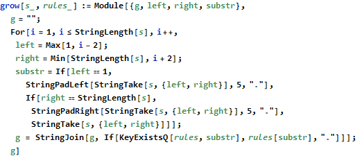
Here we apply the example rules and input. I import the rules as a table separated by the delimiter “ => “ and skip the first two lines. In retrospect, I probably could have used ReplaceAll and achieved the same result.


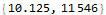
So on to part 1. We subtract 11 from the positions in the final step because I prepended 10 periods to the input and Mathematica uses 1-indexed arrays.


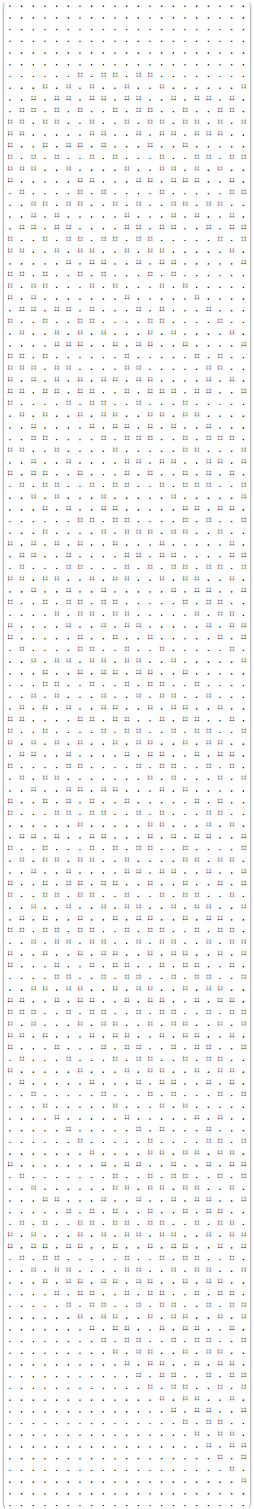


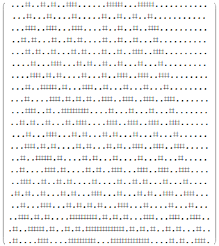
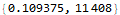
Part 2 asks us what happens after fifty billion generations -- clearly a problem that should not solved through computation alone! My instincts told me that the system might attract to some fixed point. I was wrong that the system attracts to some fixed point, but it does attract to a fixed shape.

We can see from this plot that the number of octothorpes (the “#” symbol) attracts to 73. Though the count of these symbols remains constant, their position translates in the +x direction forever. We see that the sum of positions attract to a straight line after about 120 iterations.

Since these points form a line we can a linear regression to find their total after fifty billion generations. There might be a more elegant way to combine the range [120,150] with the position sum of octothorpe symbols at the corresponding

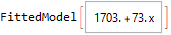


Imagine my surprise when the AoC website told me this answer was too low. It turns out that the decimal numbers given by the fitted model do not give enough precision to correctly answer the question. Mathematica calculates approximate numerical results on inputs containing an explicit decimal point. Mathematica gives an exact result when we provide our input without the decimal points.


Day 13
I’m intimidated of even thinking about day 13 again. Day 13 is another particle simulation, only this time the particles follow a finite set of paths and we have to worry about collisions. There are many rules to consider and I was never able to produce a correct answer for part 2, despite several attempts. Mathematica didn’t seem especially well-suited to this task. The problem is naturally stateful; you can use functional programming, but the object-oriented approach seems more intuitive.
I used angles and trigonometric functions to model sled direction -- to my detriment. The models are displayed in a zero-indexed world with the origin at the top-left of the screen and descending positive y-axis. Matching the “^” and “v” symbols from the input to this world is confusing and error-prone. It would have been easier to have manually precomputed direction changes as down values in a lookup table (function) instead of using sine and cosine. I did make use of down values when transitioning states because I couldn’t think of a clever function to model the cycle f(-1)=0→f(0)=1→f(1)=-1.
A further frustration with Mathematica is that the language is 1-indexed (the problem expects a 0-index world) and matrices are interpreted in row-major order. An m×n matrix has m rows; this can be really confusing if you intended to model (x,y) coordinates in column-major (x columns).
Crossroads (“+“), negative turns (“/”), and positive turns (“\”) are read and stored in a sparse array named “allturns.” I initially missed the instruction to tick each sled one at a time (in reading order). This implies that the input “>>” causes a collision; the left sled ticks and collides before the right sled can move out of the way.
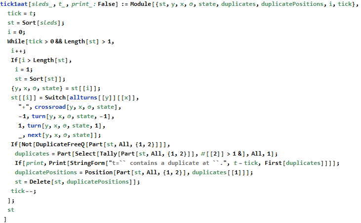
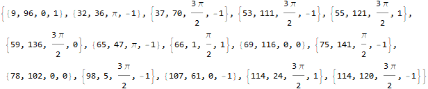
This ugly function ticks the input t times and returns the resulting list of sleds along with their orientation and state. A useful aspect of this approach is that the data is already serialized into a portable format.

At t=3234 we discover the first collision at x=129 and y=50.


This algorithm does not compute the correct answer for part 2.

Day 16
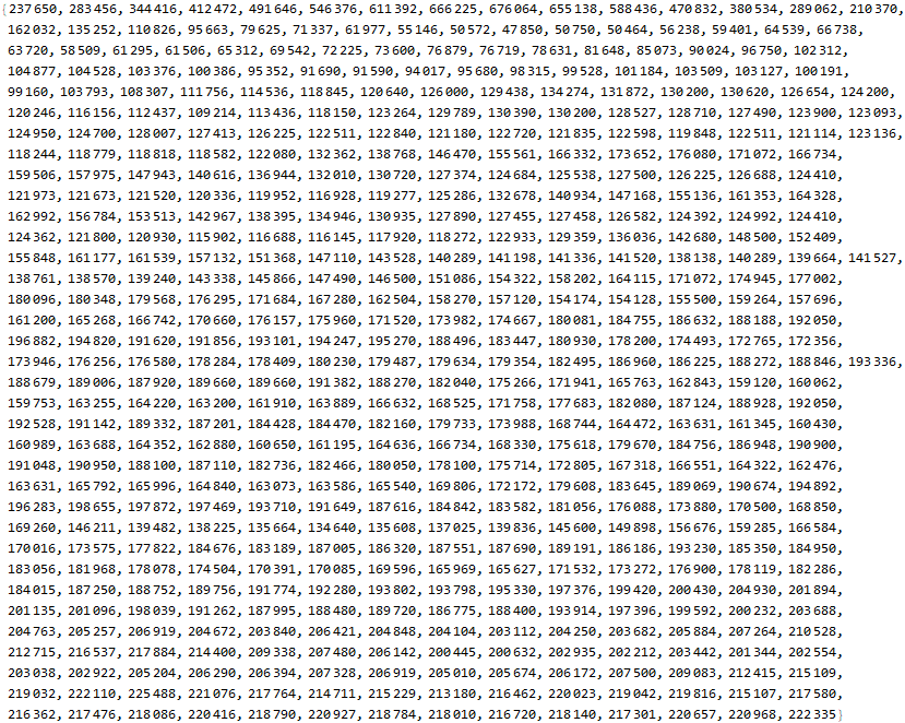
Day 16 is the first of three days where we are prompted to implement and interpret and assembly language. Some participants on Reddit unofficially call this ISA “elfcode.” All instructions consist of four values: an opcode, two inputs (A and B), and output register (C). There are four registers (0-3) and sixteen opcodes (0-15). The numeric opcode associated with each named instruction is not given.
I took the same functional approach to building my virtual machine for day 16 that I used in day 13; my virtual machine accepts an instruction (a list) and a set of register values (another list) and returns the resulting set of registers (yet another list). This approach is slow but easy to analyze and troubleshoot.
I use a light abstraction layer to save on typing; each instruction accepts either two registers, one register and one immediate value, or one immediate value and one register. The rrInst, irInst, and riInst prototypes each accept a function that it will perform against the inputs A and B. All instructions end up writing to some register C, so I consolidate this change by calling the seti function internally.

The first part of the problem has us count the number of input, instruction, and outputs possible using three or more instructions.
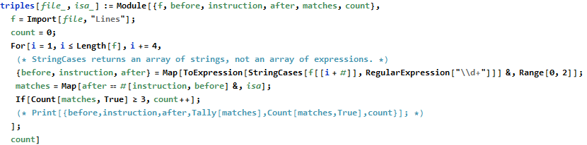


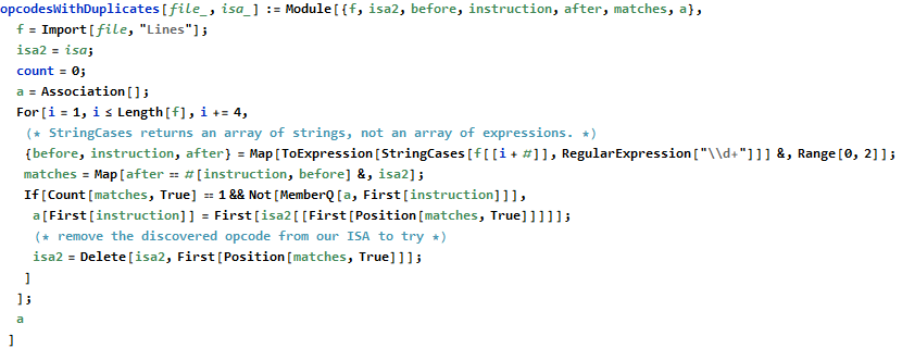
The next part of the problem has us figure out what each opcode actually does and then execute a program in our virtual machine. Finding the correct opcode is not difficult. The idea is to try all sixteen functions on a given input. If only one instruction produces the expected output then we know which instruction that is. The input only contains enough information to uniquely identify a single (14=muli). From there, we remove muli from our set of testable instructions and eventually find that 13=addi. Continue until all instructions are known.


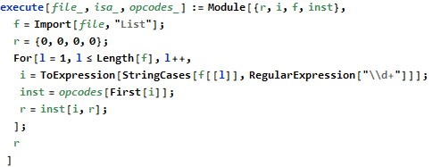
Now that we have a usable set of opcodes we can execute the program and read the result in register 0.


I am not strong on assembly languages so these low-level programs were fun, interesting, and challenging. There was a similar problem last year (https://twitter.com/wjholdentech/status/944832433211375616) that I also enjoyed.
Day 18
Another cellular automata problem.
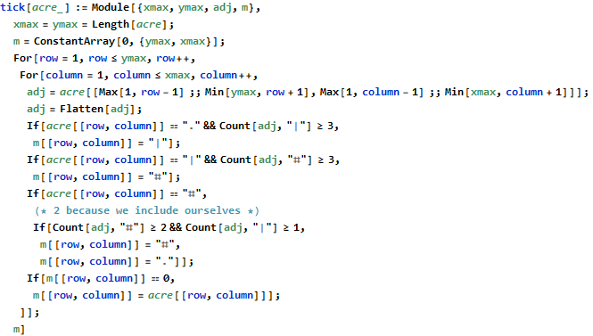
We reproduce the examples given and make use of the Nest function to apply “tick” to the input 10 times.


Now for the puzzle input:


For part 2 we are prompted to repeat this process a billion times. Reminiscent of day 12, we assume the system attracts to either a fixed point or cycle and search for a non-computational solution. (At this point I feel obligated to mention that this solution is the result of hours of hard work; I did not arrive at this answer on the first attempt.)

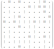
We see that the system attracts somewhere around 500. We can easily spot the cycle in the below output.


The period length for our cycle is 28. We use the modulus operator to find the relative position in the cycle that one billion will be at to find our answer.


Day 19
Another adventure in assembly language. Day 19 adds an instruction pointer (IP) and two additional registers. I didn’t have to modify my instructions from day 16 at all. All I needed to do was enhance the loop reading and executing instructions to also handle the new IP and halt when IP extends beyond the program length.
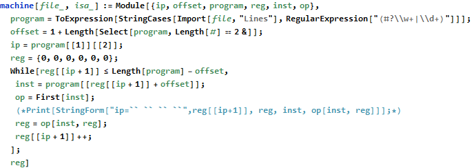
Not fast, but it computes the correct answer.


Part 2 has us set register 0 to the value of 1 and re-run the program. Sounds straightforward, right? I think most people set the register and happily wait for a result. And wait. And wait. Eventually I, like everyone, realized that something was wrong and we needed to take a closer look.
I didn’t immediately try to decipher the instructions. Instead, I extended the earlier virtual machine to print instructions and accept arbitrary register assignments as a parameter.
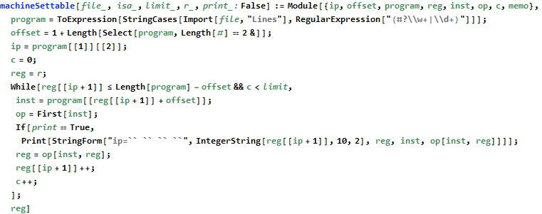
This is useful to peek inside what the program does and try to figure out how it works.


The program appears to get stuck in a loop at instructions 3-6 and 8-11 and skips instruction 7. A closer analysis of the behavior and source code indicates that the program is not trapped in an infinite loop, just a very large loop. Register 0 is being used as some kind of running total, calculated in increments of register 2. Register 1 is the instruction pointer. Register 2 is used as an outside loop counter and register 3 is used as an inside loop counter. Register 4 is used for relation tests and register 5 is some calculated constant 10551296.
By studying values that change register 0 I determined that this program is finding the sum of divisors of 10551296 through a brutal  pair of nested loops.


At some point I implemented the same virtual machine in Java before I figured out what this “quadratic nightmare” actually does. My Java-based virtual machine runs many orders of magnitude faster (something crazy, like a million times faster) it is still not fast enough to execute a trillion virtual instructions in a realistic time.
Day 21
Day 21 returns us to the same assembly language for the third and final time. We are asked what input in register 0 can terminate the given program in the fewest instructions. Analysis of the source code reveals that the program terminates at line 28 if and only if register 0 and register 5 are equal. By modifying the machineSettable function to print instructions at line 28 we see the first value the program compares.
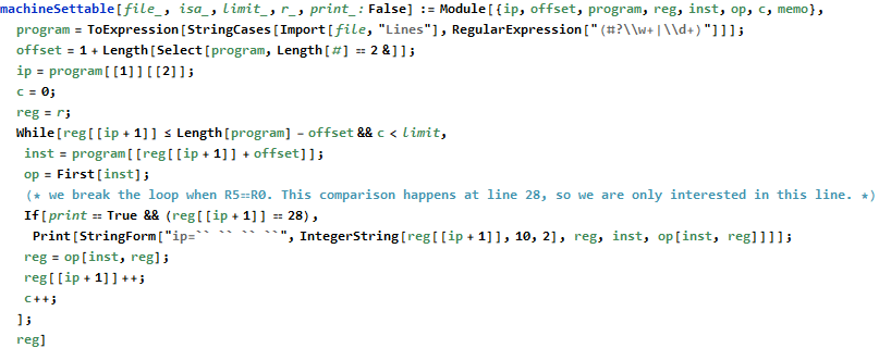


The value 2884703 is our answer; if entered into register 0 the program would terminate.
I never solved part 2 of this program. Part 2 asks us to find the value for register 0 that would cause the program to terminate after the most instructions. I studied the assembly code for quite a while and never did recognize what this program actually does.
Day 22
Day 22 is a graph problem with an interesting twist: the path cost depends on the “equipment” you are using. I spent hours and hours on this problem and solved part 1 but never correctly answered part 2.
The first part is another submatrix summation problem. The “smallest rectangle that includes 0,0 and the target’s coordinates” is obviously the rectangle with opposite corners (0,0) and (x,y). The value of at each point is given by a doubly-recursive function, geologicIndex.

As we see, recreating just a small portion of the sample input takes quite a while. We can speed this up with dynamic programming. Mathematica’s syntax allows us to easily memoize function calls as down values.

Now the result of the doubly-recursive call will be cached. The function is now very fast.

Now to compute part 1 we substitute in the input values and find the area sum.

I explored many approaches to part 2. It pains me that I work in computer networking and failed to solve this problem. I ended up writing my pathfinding problem in Java but made a fatal algorithmic mistake. I write about my experience here as an example of what not to do in this problem.
My approach was to perform a breadth-first search, enqueuing explorations from point (x,y) to point (x±1,y±1) only if δ(x±1,y±1)>δ(x,y)+d((x,y),(x±1,y±1)). That is, reexplore an adjacent point (x±1,y±1) only if the distance from the origin to (x,y) plus the distance from (x,y) to (x±1,y±1) is less than the previously known distance from the origin to (x±1,y±1). It’s like a non-greedy (and therefore slow) variant of Dijkstra’s algorithm. My algorithm kept three δ values for each coordinate. Each δ value corresponded to the path cost if using the torch, climbing gear, or neither. If the terrain was incompatible with a tool then that δ value would always be set to an infinite distance.
To my frustration, my algorithm computed the correct path cost for the example input but not the puzzle input. The problem was that the function to transition state did account for tool transitions when moving across three different types of terrain. I have not looked closely at the solutions others came up with. I saw mentions of vanila Dijkstra and A* algorithm use across two dimensions. This sounds very interesting.
Day 23
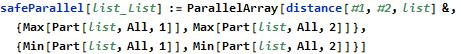
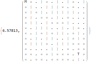
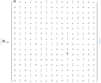
Day 23 was the last day that I worked on AoC this year, both because of family commitments and burnout from days 21 and 22. Day 23 starts with a straightforward geometry question where we are asked to find number of nanobots within range of the one with strongest signal using Manhattan distance.


I was not able to solve part 2, and from a cursory look at Reddit it sounds like this problem required the deepest math of any AoC problem this year. I assumed that the solution would surely occur at a center point or corner. I calculated the number of nanobots in range from each of these 7000 points and took the greatest of these. Wrong answer, but hey look at this cool visualization:


Summary
Advent of Code is one of the best resources out there for learning to program. These problems got very hard and it was an incredibly humbling experience for me. The competitive aspect is not interesting to me; some people solve these problems in less time than it takes me to read the problem description. Impressive, but I trust these talented people leave their speed tricks at home when they work on professional software. Other programmers came up with incredibly elegant, clever, and efficient solutions to problems that I would probably never have found. Some incredible souls wrote their AoC solutions in a different programming language every day. This is just stunning.
In another way, though, AoC boosted my confidence in some ways. I think that at least a few of my programs in this document are halfway decent. I learned a lot about Mathematica and scratched the surface of the functional programming iceberg. I wasn’t the only person who thought AoC was very difficult this year and I got to apply some of the skills (especially dynamic programming) that I’ve learned over the past year on edX.
My favorite aspect of AoC is not the programming challenges themselves, not the competitive aspect, not the Christmas theme -- it’s the community. The AoC community is incredibly supportive and friendly. AoC attracts a huge community that focuses very hard on a single crazy problem on one day and openly shares solutions, unlike university computer science classes. This year we saw many compelling visualizations; my favorite was this visualization of the Elves and Goblins fighting in Unity (https://www.reddit.com/r/adventofcode/comments/a6sej7/day_15_unity _visualization/). I have been frustrated with the algorithms courses I have taken on edX because they do not allow you to share code. I understand why but I think I could learn a lot both from reading and explaining solutions.
Project Euler (https://projecteuler.net) is another resource with programming problems. Where most of AoC’s problems are solvable through brute force (and some are only solvable through computation), many of Project Euler’s problems are only solvable through higher mathematics. Project Euler unlocks a forum to discuss solutions once someone solves the problem. It is an interesting middle ground. AoC leaves the solutions available to everyone. Colleges discourage collaboration on individual assignments. I think AoC’s open approach is the best way to learn when you simply don’t know what you don’t know.
In the next year I hope to finish this program I’ve been taking on edX and get serious about learning Python. Mathematica is a powerful and useful tool; I think AoC has given me enough experience with Mathematica to better assess its fitness for a given problem.
I hope this writeup is useful to someone. I am obviously very far from being an expert, but occasionally people learn better from peers than professors (which is why we have TAs in college). I will be very interested to read reflection papers by others. Merry Christmas and have a happy new year!